With the help of ML frameworks, AI is experiencing tremendous growth in bridging the gap between machines and humans. The progress in computer vision and image recognition has been due to the creation and smooth implementation of Convectional Neural Networks (CNNs). CNN enables Deep Learning, which is a division of Machine Learning. This tutorial explains a convolutional neural network and how to train an algorithm using CNN technology to classify CIFAR images.
What Is Convolutional Neural Network (CNN)?
Convolutional Neural Networks (CNN) is a specialized category of artificial neural networks that helps recognize images and enable understanding of computer vision because of its specially designed processing of pixel data. CNN algorithms enable robust image processing power that allows deep learning models to achieve generative and descriptive jobs, often using machine vision (camera). It can recognize images and videos through an effective learning mechanism and acts as a recommender system. Computer vision also helps in (Natural Language Processing) NLP by understanding the number or letter/word written in an image and parses it into machine-understandable meaning. The main difference between a Convolutional neural network and other types of neural networks is that it takes all its inputs as a 2D array. Also, it performs its operation directly on the images rather than concentrating on feature extraction done by other neural networks. CNN implementation includes explanations and solves problems of recognition. Top multi-national giants like Google, Microsoft, Facebook, etc., have sponsored heavily in research and development (R&D) into practical projects to get activities done with incredible pace. CNN caters to three basic ideas. These are:
- Local respective fields
- Pooling
- Convolution
How Does a Convolutional Neural Network Work?
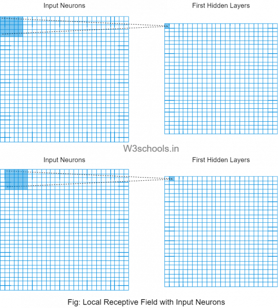
The working of a CNN is analogous to that of the connection pattern that occurs in our human brain. Each brain neuron reacts to stimuli only in a fixed visual field region. We call this the Receptive Field. A compiled cluster of such fields coincides jointly to wrap the entire visual area. Similarly, CNN employs spatial correlations that live within the input data. Each concurrent layer within the neural network links to some additional input neurons. This distinct region is called a local receptive field, which concentrates on the hidden layers of neurons. These hidden neurons are responsible for processing the data input residing within the mentioned field.
Here is a graphical representation of how the local respective fields get generated:

From the above graphical representation, we can figure out that each connection carries the weight of the neuron from the hidden layer as a link while moving from one layer to another. These individual neurons perform a shift with time, which is called "Convolution." The mapping or linking of the connections from the input layer into the hidden layer carries the "shared weight" and "shared bias" values.
TensorFlow Program to Train a CNN Model for Image Recognition
Example:
import tensorflow as tf
import matplotlib.pyplot as plt
from tensorflow.keras import datasets, models, layers

#Download and prepare the CIFAR10 dataset
(train_imgs, train_lebs), (test_imgs, test_lebs) = datasets.cifar10.load_data()

#Normalizing the pixel values by keeping it between 0 & 1
train_imgs, test_imgs = train_imgs / 255.0, test_imgs / 255.0

category_names = ['airplane', 'automobile', 'bird', 'cat', 'deer', 'dog', 'frog', 'horse', 'ship', 'truck']

#To verify that the dataset looks correct,
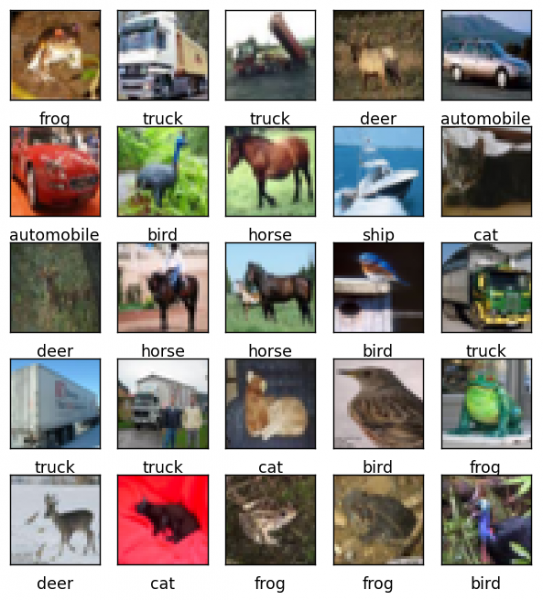
#plot the first 30 images from the training set and display the class name at the bottom of each image.
plt.figure(figsize=(8,8))
for i in range(25):
    plt.subplot(5,5,i+1)
    plt.xticks([])
    plt.yticks([])
    plt.grid(False)
    plt.imshow(train_imgs[i])
    # We have used the CIFAR labels that used to be arrays. For this we have to use extra index
    plt.xlabel(category_names[train_lebs[i][0]])
plt.show()


#Create the convolutional base
mod = models.Sequential()
mod.add(layers.Conv2D(32, (3, 3), activation = 'relu', input_shape = (32, 32, 3)))
mod.add(layers.MaxPooling2D ((2, 2)))
mod.add(layers.Conv2D(64, (3, 3), activation = 'relu'))
mod.add(layers.MaxPooling2D((2, 2)))
mod.add(layers.Conv2D(64, (3, 3), activation = 'relu'))
mod.summary() #It displays complete architecture of the model

#Add Dense layers on top
mod.add(layers.Flatten())
mod.add(layers.Dense(64, activation='relu'))
mod.add(layers.Dense(10))
mod.summary()

#Compile and train the model
mod.compile(optimizer = 'adam',
              loss = tf.keras.losses.SparseCategoricalCrossentropy(from_logits = True),
              metrics = ['accuracy'])

history = mod.fit(train_imgs, train_lebs, epochs = 10,
                    validation_data=(test_imgs, test_lebs))
Output:

Model: "sequential"
_________________________________________________________________
 Layer (type)                Output Shape              Param #
=================================================================
 conv2d (Conv2D)             (None, 30, 30, 32)        896

 max_pooling2d (MaxPooling2D  (None, 15, 15, 32)       0
 )

 conv2d_1 (Conv2D)           (None, 13, 13, 64)        18496

 max_pooling2d_1 (MaxPooling  (None, 6, 6, 64)         0
 2D)

 conv2d_2 (Conv2D)           (None, 4, 4, 64)          36928

=================================================================
Total params: 56,320
Trainable params: 56,320
Non-trainable params: 0
_________________________________________________________________
Model: "sequential"
_________________________________________________________________
 Layer (type)                Output Shape              Param #
=================================================================
 conv2d (Conv2D)             (None, 30, 30, 32)        896

 max_pooling2d (MaxPooling2D  (None, 15, 15, 32)       0
 )

 conv2d_1 (Conv2D)           (None, 13, 13, 64)        18496

 max_pooling2d_1 (MaxPooling  (None, 6, 6, 64)         0
 2D)

 conv2d_2 (Conv2D)           (None, 4, 4, 64)          36928

 flatten (Flatten)           (None, 1024)              0

 dense (Dense)               (None, 64)                65600

 dense_1 (Dense)             (None, 10)                650

=================================================================
Total params: 122,570
Trainable params: 122,570
Non-trainable params: 0
_________________________________________________________________
Epoch 1/10
1563/1563 [==============================] - 42s 27ms/step - loss: 1.5505 - accuracy: 0.4343 - val_loss: 1.3137 - val_accuracy: 0.5250
Epoch 2/10
1563/1563 [==============================] - 38s 24ms/step - loss: 1.2090 - accuracy: 0.5704 - val_loss: 1.0982 - val_accuracy: 0.6096
Epoch 3/10
1563/1563 [==============================] - 30s 19ms/step - loss: 1.0566 - accuracy: 0.6268 - val_loss: 1.0325 - val_accuracy: 0.6335
Epoch 4/10
1563/1563 [==============================] - 60s 38ms/step - loss: 0.9549 - accuracy: 0.6646 - val_loss: 1.0076 - val_accuracy: 0.6433
Epoch 5/10
1563/1563 [==============================] - 45s 29ms/step - loss: 0.8812 - accuracy: 0.6900 - val_loss: 0.9929 - val_accuracy: 0.6549
Epoch 6/10
1563/1563 [==============================] - 55s 35ms/step - loss: 0.8176 - accuracy: 0.7124 - val_loss: 0.9217 - val_accuracy: 0.6715
Epoch 7/10
1563/1563 [==============================] - 25s 16ms/step - loss: 0.7717 - accuracy: 0.7293 - val_loss: 0.8942 - val_accuracy: 0.6869
Epoch 8/10
1563/1563 [==============================] - 25s 16ms/step - loss: 0.7273 - accuracy: 0.7448 - val_loss: 0.8594 - val_accuracy: 0.7010
Epoch 9/10
1563/1563 [==============================] - 26s 16ms/step - loss: 0.6787 - accuracy: 0.7627 - val_loss: 0.9164 - val_accuracy: 0.6943
Epoch 10/10
1563/1563 [==============================] - 25s 16ms/step - loss: 0.6510 - accuracy: 0.7709 - val_loss: 0.9106 - val_accuracy: 0.6894
You will finally notice that the CNN model training will achieve an accuracy of more than 75% (shown as 0.7709).